How can I convert raw radar data in my own format into something that radR can use?

Step 1:  Create the raw archive file

This is easy:

> bl <- biglist("myrawfile.raw.biglist", overwrite=TRUE, cache.size=1, names=c("pulses", "samples.per.pulse", "bits.per.sample", "timestamp", "time.msec", "duration", "sample.dist", "first.sample.dist", "bearing", "orientation", "antenna.lat", "antenna.long"))

> bl

[1] "radR biglist object with length = 0"

If you do not use/have latitude and longitude information, omit the last two names from the call to biglist() above.

Step 2:  Create the table of contents

For each sequence of consecutive scans in your file, you need to know the dates and times of
the first and last scans, and the number of scans.
For example, suppose you know that your file has 2 sequences of scans:

1. 120 scans from Jan 15, 2006 11:30:04 to 11:33:58 (each scan lasts 2 seconds)
2. 60   scans from Jan 15, 2006 11:40:00 to 11:41:58

Then you can create the table of contents like this:

contents <- list(num.scans=c(120, 60))
times <- as.POSIXct(c("2006-01-15 11:30:04", "2006-01-15 11:33:58", "2006-01-15 11:40:00", "2006-01-15 11:41:58"))
contents$start.times = as.integer(times[c(1, 3)])
contents$end.times = as.integer(times[c(2, 4)])

and save it like this:

bl[[1]] <- contents

Step 3:  Create a scan parameter item

Items 2, 4, 6, ... in the biglist bl will contain lists of scan parameters for the raw scan data in items 3, 5, 7, ...

To create a scan parameter item, do this:

scan.info <- list (pulses = 1024,   ## this is the (constant) number of pulses in a single scan  
                                    ## See "Gating your data..." below if you have variable pulses per scan.

samples.per.pulse = 512, ## the number of samples of raw echo data from a single pulse

bits.per.sample = 12,    ##  the bit resolution of your analog to digital converter

timestamp = as.integer(as.POSIXct("2006-01-15 11:30:04")) + time.offset,
                         ## the (double) timestamp for the start
                         ## of the scan, with fractional seconds in time.offset = 400
 

duration = 2000,         ## the duration of the scan, in milliseconds

sample.dist = 5,         ## the size of a sample or range cell, in metres

first.sample.dist = 0,   ## the range at which the first sample or range cell begins;  typically zero,
                         ## but non-zero values can be used to eliminate (negative) or insert (positive)
                         ## a hole at the origin, to account for incorrectly set trigger delay / cable length
                         ## or selective digitization.  (Note: as of October 2008, non-zero values are not yet                              ## supported. Please contact the author if you would find this feature useful.)

bearing = 0,             ## the direction of the first pulse in the scan, in degrees clockwise from north

orientation = 1,         ## the radar scan direction (viewed from above):  +1 = clockwise, -1 = counterclockwise

latitude = 45.5545,      ## the antenna latitude, in degrees North (optional)

longitude = 120          ## the antenna longitude, in degrees West (optional)

)

 And to store it as the parameter list for the first scan, do this:

    bl[[2]] <- scan.info

Step 4:  Create a raw scan data item

There are many ways in which to do this, depending on how you got your raw data into R.
In what follows, we assume these variables have been assigned:

pulses <-  number of pulses in the scan ## This should be constant across scans; see "Gating your data..." below
spp    <-  number of samples per pulse
bps    <-  bits per sample

Here are some possibilities:

 

Data in an R double vector, x, with each element representing one sample, and an arbitrary range of values:

x <-  as.integer(65535 * (x - min(x)) / (max.x - min.x))
rawscan <- .Call("raw_pack", x, c(4, pulses * spp, bps, .Platform$endian == "big"))

Data in an R integer vector, x, with each element representing one sample:

rawscan <- .Call("raw_pack", x - min.x, c(4, pulses * spp, bps, .Platform$endian == "big"))

Data in an R raw vector, x, with 12-bit samples each occupying 2 bytes, so that sample 0xabc is represented by 0xbc followed by 0x0a:

rawscan <- .Call("raw_pack", x, c(2, pulses * spp, bps, .Platform$endian == "big"))

In all cases, min.x and max.x must be the minimum and maximum of all possible sample values, not just the minimum and maximum in a particular scan.  And in all cases, pulses and samples within pulses are in order from earliest to latest, and there is no padding between pulses. For other cases, contact the author.  Note: radR can only use unsigned integer data with at most 16 bits per sample.The first example above shows how to rescale your data to fully use the 16 bits of resolution.

Once you have obtained the raw data, here is how to store it in the raw archive:

bl[[3]] <- rawscan

Step 5: repeat, and then close the file

You will need to repeat steps 3 and 4 for each scan of data.  Scan info and scan data are stored in the order corresponding
to the table of contents:  first those from the first segment, then those from the second segment, and so on.
When you have written out all scan info and data items, flush and close the biglist as so:

close(bl)  ## forces everything to be written to disk, and releases file connections

If everything worked, you will have two files: myrawfile.raw.biglist and myrawfile.raw.biglist.i
You should be able to read these into radR using the "From: -> raw archive" button in the player window.

 Step 6: testing your file

Before converting large data sets, try this from the radR console window so that you are sure parameters have been chosen and that no bug in this documentation or in radR is causing problems:

bl <- biglist("myrawfile.raw.biglist", read.only=TRUE)   ## open the newly created raw biglist
si<-bl[[2]]                                             ## read a scan info record to obtain scan data size
rdat<-bl[[3]]                                            ## read the packed raw data into a character scalar
dat<-matrix(integer(0), nrow=si$samples.per.pulse,       ## allocate space for unpacked data
ncol=si$pulses)
invisible(.Call("raw_unpack", rdat, dat,                 ## unpack the data (&apos;invisible&apos; suppresses its display)
          c(4, si$pulses * si$samples.per.pulse,
si$bits.per.sample, .Platform$endian == "big")))
plot(dat[,1], pch=".")                                   ## this should be the plot of all samples from a single pulse
close(bl)

Troubleshooting

If your data look funny when you open them in radR, it may be that you have used a 4 instead of a 2 or vice versa, in this line:

rawscan <- .Call("raw_pack", x, c(4, ...

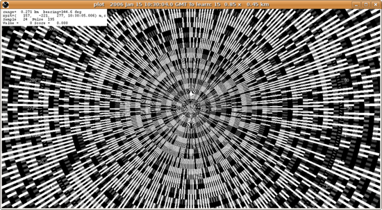
Using a 2 when a 4 is required will cause data in the plot window (when zoomed in toward the origin) to look like this:

i.e. there seem to be holes between pulses and samples.
Note also that there are some many bright samples immediately beside very faint ones.
This is probably due to converting negative data, which radR cannot yet use.  Before creating the raw archive, you should scale your data so that the minimum value is 0: 

x <- x - min(x)
 

(The very bright samples arise from interpreting small negative integers as large unsigned integers.)

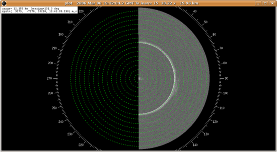
Using a 4 when a 2 is required will cause data in the plot window (when zoomed in toward the origin) to look like this:


i.e. only half the scan has data, and the bright clutter from near the radar is repeated at half the maximum range.

Gating your data to achieve constant pulses per scan

If radR crashes when viewing your data, it might be because the number of pulses per scan is not constant.  [In the future, radR will handle this, but it is a bug as of revision 59.]
You can use a simple gating function to duplicate/drop pulses for each scan as required:

m <- dim(dat)[2] ## dat is the matrix of non-negative integer sample values from one scan
n <- 486         ## n is the desired constant number of pulses per scan; pick a number suitable for your data

## for each desired pulse, use the closest actual pulse:
dat <- dat[,1 + round((0:(m-1)) * n / m)]

## now call raw_pack and write the data to the appropriate biglist slot...

If you have the empirical azimuth for each pulse, a more correct  method of gating can be achieved with R&apos;s approx() function:
    m <- dim(dat)[2]           ## dat is the matrix of non-negative integer sample values from one scan
    n <- 486                   ## n is the desired constant number of pulses per scan; pick a number suitable for your data
    stopifnot(length(h) == m)  ## h is the heading for each pulse in dat; units are degrees clockwise from North;
                               ## h must have one element for each pulse, but elements can be "NA" for pulses with
                               ## no angle measurement.  We assume the first pulse has heading 0; i.e. North.

    ## For each desired pulse azimuth, use the closest actual pulse, interpolating linearly from empirical headings.
    ## We add a virtual copy of the first pulse so that interpolation works correctly for angles close to 360 degrees.

    dat <- dat[, round(approx(x = c(h / 360, 1), y = c(1:m, 1), xout = (0:(n-1)) / n, method="linear", rule=2)$y)]

    ## now call raw_pack and write the data to the appropriate biglist slot...